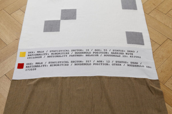
Rossella Biscotti, Detail of Dead Minorities, 10×10 series, 2013, jacquard woven textile, courtesy of the artist

Introduction

Other began as an ongoing project initiated for the exhibition 10 x 10 (2014), which was presented at Haus Esters in Krefeld, a modernist villa designed by Ludwig Mies van der Rohe for the silk manufacturer Josef Esters. In an exploration of how institutional structures are imposed on individuals, the first textile series combines features of automated mechanical manufacturing with conceptual and technological aspects of how large datasets are collected and processed.

Haus Esters was built in a classical family structure with a family room, a man’s room, a woman’s room, and a children’s room. With this rather traditional idea of how a family is composed as a starting point, we looked at the definition of households within the population census of Brussels. We examined the lives and relationships within different households included in this dataset and ultimately replotted this demographic analysis into the form of woven textiles.

Unfolding the census and all its information, we navigated different relationships and typologies defining the social position of an individual and its relation to this population. Our focus was on how categories are used to create an overarching structure, which we related to punch cards—a binary system of programming used to implement such structures within industrial and administrative processes that became increasingly automated in the early 20^th Century, namely the Hollerith machine for early data processing and the automated Jacquard Loom for weaving textiles.

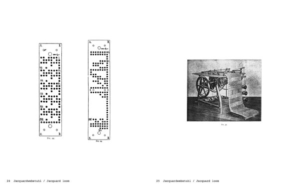
Jacquard loom

We looked at the communication and translation of complex constructions within a simplified system setting. In the census, an individual’s status is determined by his or her answers to a hierarchical flow chart of “yes” or “no” marital enquiries that are centered on the criteria of a conventional family unit. “Other” is the last box: a category of people that have “fallen out” of all given possibilities. For example, a person sharing an apartment with a fellow student or co-worker; a grandparent hosted by a different family; or people in temporary living conditions. Investigating this label, we focused on different groups that contained one or more relationships or positions defined as “other”, tracking different relational behaviours that run through the census as a pattern. These four focused datasets—Other (44-person household), Other (60-person household), Other (current residents), Other (former residents)—are the conceptual base for the installation shown within Contour Biennale 8.

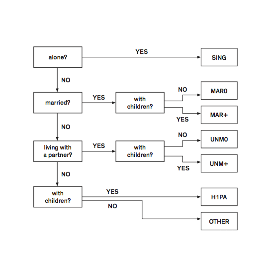
Household Position Flow Chart, Brussels 2001 Census / These questions are used to define the marital status of queried individuals

The textiles are a matrix composed of square modules where “x” and “y” are given conditions and “z” is the quantity of individuals placed in the same position. These quantities are represented by a grayscale, created through different woven bindings (where black is the highest density of people and white the lowest). Some individuals are singled out and their data re-emerges in textual form on the bottom of the matrix. This form of data montage establishes an intrinsic relationship between “official” power structures and “unofficial” individual narratives. We traced and analysed how a person’s residential status remains static or fluctuates—how an individual might be reabsorbed into a family structure, disappear, move away from the city, or die.

“Other” as default (or empty label)

The series Other investigates further an ambivalence between the position of the individual within society and the generalisation of this individuality within a system of predefined typologies, creating an arbitrary narrative of a subject’s life or history. The subject carrying the label “other” can be considered as default: a value representing nothing but itself, and positioning itself on the peripheries of the total or generalisation of a big dataset. The term “default” can signify two essential, contrasting meanings:

1. Default as failing or failure; omission of that which ought to be done.

2. Default as a value used when none has been given; a tentative value or standard that is presumed.

The individuals in this group become the misleading entities that fall out of a defined frame and as such, demarcate interstitial spaces of non-information. In contrast to the first position, a default is also defined as a pre-set value or position given in an automatic way. The label “other” quickly becomes the definition of a “rest” group, where the information is known but its relevance isn’t included in the general image. The complexity of this rest-group stems from individuals being grouped together based on their dissimilarities, rather than their similarities.

Looking at the different typologies within current society and its variety of relationships, it seemed appropriate to create a dialogue between the visualisation approach and a more analytical understanding of “other.” Whereas the installation work reflects on the tension between individual and collective structures and on the loss of individuality caused by data aggregation, here we restrict our attention to the informational significance of labels like “other.”

Rossella Biscotti, Other series, 2014, installation view at Contour Biennale 8. Courtesy of the artist and Contour. Photo: Kristof Vrancken

We investigate the understanding of “other” and similar labels as semantically or informationally empty labels. That is, labels that can be used for the sake of convenience, for instance to flag something, but which do not attribute a property. Using one type of terminology, we will say that such labels do not indicate membership in a category; using another terminology, we will say they do not assign a type. This kind of understanding of “other” as a mere label is analogous to the use of so-called sentinel values like NaN (not a number).

Labels like “other” can be assigned because certain data subjects do not belong to any of the categories chosen by the designers of a census, or perhaps because the subjects belong to a category that is too small to be of any practical importance. The former understanding applies to variable “household position,” where “other” results from negative answers to four consecutive yes/no-questions. The latter applies to nationalities or statistical sectors whose prevalence in the dataset is small (e.g. under 100), and which are therefore lumped together.

We use the terms “type” and “token” to refer to, respectively, properties and the concrete entities to which properties are attributed. When applied to census data, tokens should be understood as data subjects or persons, and types as (integer or categorical) features. To zoom in on the meaning of “other,” we will also talk about the attribution of labels to tokens.

Once types are assigned to tokens, tokens can be compared in terms of how similar they are, or even how they are aggregated. Being of the same type, or sharing a type, indicates a certain kind of similarity; a shared property. An interesting way to understand “other” is precisely as a label that does not signal any similarity among the tokens that receive that label. “Other” does not correspond to a type because it does not attribute a property. Indeed, negative answers to a series questions cannot indicate the same kind of similarity as positive answers to such questions. Given these considerations, we can investigate how the presence of empty labels affects the identification of similar groups within a set of tokens, and specifically within a population, and explain the informational role of such labels in terms of their effect on the identification of groups with similar features.

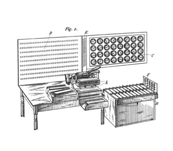
Hollerith, tabulating machine

Abstract Classifications

Before we consider specific data, we will first consider the concept of empty labels in a purely abstract setting, and highlight some features within some toy examples. We will start with a few definitions based on Barwise and Seligman (1997):

Definition 1 (Classification) A classification   consists of a set of tokens, a set of types, and a binary relation between them.

Definition 2 (Invariant) Given a classification A, an invariant is a pair (Σ, R) with Σ ⊆ tok(A) and         R ⊆ tok(A) × tok(A) such that aRb holds if: Given the definition of R, it is easy to see that an invariant defines an equivalence-relation. We will henceforth write a ≡ b whenever aRb holds Σ in view of the invariant (Σ, R) on A.

Definition 3 (Quotient) Where I = ⟨Σ, R⟩ is an invariant on A, we write A/I to denote the quotient of A by I where:

1. typ(A/I) = Σ (the types are inherited from the invariant),

2. tok(A/I) are the ≡ -equivalence classes [a] obtained from tok(A), Σ Σ

3. 

With invariants and quotients so defined, we can show how a classification can be used to make abstractions from individual tokens by focusing on the types shared by different tokens. Consider the following example:

Example 1. Let C1 = ⟨tok(C1), typ(C1)⟩ be a classification with tok(C1) = {1,2,3,4,5} and typ(C1 ={a,b,c,d} such that:

Intuitively, within this classification, we can say that 1, 2, 3, 5 are all of type b and thus similar in one respect, whereas 1,2,4 are all of type a and thus similar in another respect. If we want to generalise such claims, we can either take into account the types that tokens share, or (more generally) take into account the types on which tokens agree. On the former accounts, 1 and 2 share {a, b}; on the latter account, 1 and 3 agree on {b, c, d}, while they disagree on a. Both types of similarity are depicted in Figure 1, where the width of each edge indicates the degree of similarity of two tokens. For present purposes we can focus on the latter understanding of similarity, which coincided condition (†) of Definition 2.

If we now define the invariant I = ⟨{c},R⟩, we obtain 1 ≡{c} 3 and 2 ≡{c} 4 ≡{c} 5, this invariant can then be used to construct C1/I with [1]≡{c} and[2]≡{c} as the only two tokens; the token of type c and the token without type c.

One way to understand the construction of quotients is that it creates a new classification where the tokens are now (reified) categories rather than individuals or other concrete entities. The abstract classifications used in this note provide a minimal formal setting in which the effect of epistemic practices like abstraction and aggregation can be represented. Similarly, the construction of invariants based on subsets of types can be used to formally represent what happens when we make abstractions of certain types.

A consequence of the above approach that more directly addresses our core concern of the meaning of “other” is the fact that, even if we do not introduce a dedicated type for “other,” type-less tokens inevitably end up in the same equivalence-class, irrespective of the invariant one chooses. This is because (†) holds vacuously whenever for all α ∈ Σ we have  all other tokens agree on being type-less.

By adopting a stronger criterion which requires at least one type as a witness for the similarity of two tokens, such vacuous cases can be excluded:

(‡)

A second example based on a slightly more involved classification can illustrate the use of (‡).

Example 2. For this example, we use types that are more closely related to numerical or categorical features in a dataset. The classification C2 has {foo, bar, baz, bak, lol} as tokens, and {a0, a1, a2, b0, b1, c0, c1} as types, and could be seen as the result of combining three smaller classifications with: typ(C2a ) = {0, 1, 2}, typ(C2b ) = {0, 1}, typ(C2c ) = {0, 1}.

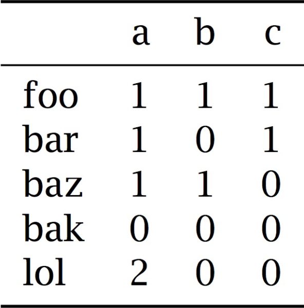
We use a table to list which tokens are of which type. This allows us to think of each column as one of the smaller classifications C2a , C2b , C2c , and it clarifies in which sense we may think of a dataset in a tabular form as an abstract classification.

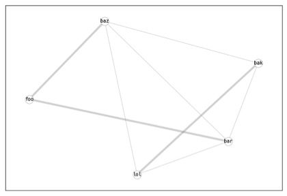
[b].5 [fig:C2left]

[b]. 5 [fig:C2right]

Figure 2 depicts the similarity (in the sense of (†)), as well as the extension of the equivalence-relation ≡Σ with Σ = {a0, a1, a2, b0, b1}. (Note: In the first case we consider how much agreement there is on all the types; in the second case we consider perfect agreement on a subset of all the types.) Here, we see that foo and baz are both of type a1 and b0, whereas the remaining tokens are, respectively, of types a1, b1, a2, b1, and a1, b0 and thus non-equivalent relative to Σ = {a, b}. In this case, the resulting equivalence-relation ≡Σ is identical to ≡typ(C2−) with C2− the result of combining C2a with C2b.

Representing Missing Types

So far, because our example does not include type-less tokens, the difference between (†) and (‡) is immaterial. If, however, we would now treat each occurrence of a 0 in the table above as a label that indicates the absence of a type, we can consider the effect of missing types on equivalence-relations.

Example 3. Consider the classification C3 with the same tokens as C2 and the restricted set of types {a1, a2, b1, c1}.

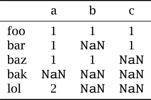
As before, we use a table to list the types of each token and use an explicit sentinel value to highlight that (what was previously) zero is no longer considered a type.

In C2 bak agrees on one or more types with some of the other tokens, but in C3 bak is not of any type, and thus cannot be similar to any other token of the classification. This is depicted in the left-hand diagram of Figure 3. If, as before, we make an abstraction of all the c-types and look at the extension of ≡Σ with Σ = {a1,a2,b1}, only foo and baz remain in full agreement.

[b].5 [fig:C3left]

[b].5 [fig:C3right]

This provides us with the necessary, although extremely basic, formal machinery to reason about empty labels such as “other.”

To clarify in a last example, we use a randomly generated dataset similar to the data used for the woven objects, so the difference between the two types of approaches taken to investigate “others” can easily be visualised. In the figures below, the sizes of categories are displayed as bubbles; the figure on the left uses the number 10 to denote “other” (and 10==10 evaluates to True), whereas the figure on the right uses NaN.

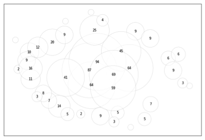
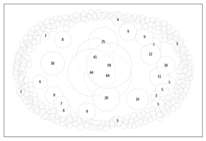
We immediately see that the presence of data subjects labelled “other” leads to a large periphery of different (because unknown) data subjects whenever the label used to denote rest-categories indicates the absence of information. This lends a preliminary understanding of how the meaning we assign to labels used to denote categories interacts with the process of creating categories or profiles, and of the subsequent use of these categories as an ontology used to describe a given subject matter.

The research on OTHER was made possible by Julia Reist in collaboration with Patrick Allo and the VUB, Brussels

The text was written in collaboration of Rossella Biscotti, Julia Reist and Patrick Allo